Introduction

After Unity has introduced its Scriptable Render Pipeline framework, I’ve been using it to develop my own experiment renderer in Unity. By utilizing SRP, we can get rid of annoying RHI abstraction work and pay attention to actually re-create techs in Unity. Now, let’s talk about PBR. There are tons of articles about PBR nowadays. I’ve read a bunch of them, but hey, it is rendering, you gotta do it to have a better understanding. As I’m trying to implement a better temporal anti-aliasing solution in SRP, it is time for me to implement PBR first to create rich specular/shading aliasing. With that being said, I’m not really doing a full physically based render pipeline. We’re still missing core features such as physical camera simulation and light that follows photometry & radiometry units.

This article is a record of my journey to implement PBR in SRP – will involve some SRP related contents.

Related Articles & References

First off, here are the resources I read to learn about PBR and SRP.

PBR Resources

1. The classic Moving Frostbite to Physically Based Rendering
2. Google’s Filament renderer and its PBR white paper. It explained many details of the Frostbite implementation, as well as given their own improvements (such as multiscattering compensation).
3. Here’s another tech blog I found on the internet (written in Chinese), as well as this one. According to my understanding, there are some mistakes in the codes & articles, but the explanation is really clear.
4. Finally, the good old learn open gl’s tutorial on PBR. I mainly read the part about image based lighting.
5. Besides, Unity also includes many utility functions to use under the shader library of the core render pipeline package. You can check BSDF.hlsl, CommonMaterial.hlsl, ImageBasedLighting.hlsl, Sampling.hlsl and etc. I didn’t use them in the end, but they are good reference points.

SRP Resources

1. Catlike coding’s Custom SRP Tutorials is a nice start to know the basics of SRP framework. But the render pipeline it teaches you to build fairly simple.
2. Then Unity also has its own SRP documentations. Be aware that many of the sample code snippets are not update-to-date and do not take account of recent API changes.
3. When you are unsure about certain engineering designs, you can simply read URP & HDRP’s source codes. The concept is kinda clear, though it might not be the best way.

PBR Implementation Journey

Roughness or Perceptual Roughness?

It was quite confusing at first on the following concepts: smoothness, roughness, linear roughness, and perceptual roughness. When I read Frostbite’s pbr docs, the values in the formulae or codes are sometimes roughness, and sometimes perceptual roughess, which is hard to distinguish at first.

Well, in fact it doesn’t take too long to understand them all. Linear roughness or perceptual roughness is the roughness value we assign when paint the PBR textures. However, it is intuitive to think that smoother surface is brighter (closer to white), so in Frostbite, we use smoothness instead of roughness. Thus, linear roughness or perceptual roughness equals to 1 - smoothness.

Meanwhile, when a surface is already very rough, the increase in roughness will be very subtle. The roughness sensitivity is high when roughness value is low, and the sensitivity is low when roughness value is high. To cope with it, Frostbite introduces a roughness remapping procedure. Instead of directly assigning linear roughness value to the alpha coefficient used in microfacet brdf formula, we use alpha = roughness = (linear roughness) ^ 2. Thus, alpha^2 = roughness ^ 2 = (linear roughness) ^ 4. Of course, there are many ways to do roughness remapping. For example, Crytek uses alpha ^ 2 = (1 - 0.7 smoothness) ^ 6, which has a close visual result compared to Frostbite’s quadratic method. Here’s an illustration from Frostbite’s docs: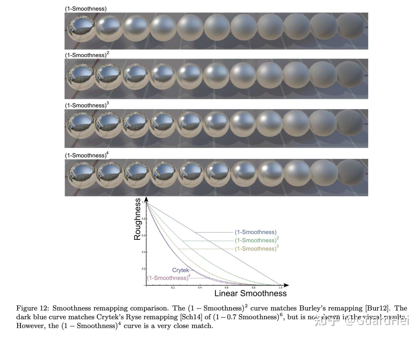

BRDF Assembly

Now, it’s time to assemble up our PBR shading function! There are 4 parts: direct diffuse, direct specular, indirect diffuse, and indirect specular. It’s like assembling up LEGO bricks, which is quite interesting.

Direct Diffuse

We could use the classic lambert diffuse model, but it is far away from an accurate representation. Here, I first referenced Frostbite’s Renormalized Disney Diffuse BRDF. The original Disney diffuse BRDF does not achieve energy conservation when linear roughness and view angle are both high (energy is larger than 1), as shown below: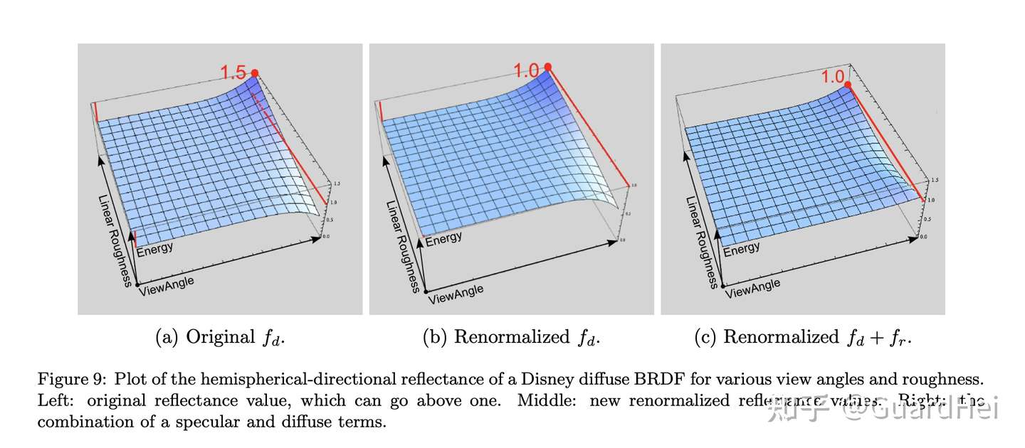

// Caller needs to div by PI
float3 DisneyDiffuseRenormalized(float NdotV, float NdotL, float LdotH, float linearRoughness, float3 diffuse) {
    float energyBias = lerp(.0f, .5f, linearRoughness);
    float energyFactor = lerp(1.0f, 1.0f / 1.51f, linearRoughness);
    float f90 = energyBias + 2.0f * LdotH * LdotH * linearRoughness;
    const float3 f0 = float3(1.0f, 1.0f, 1.0f);
    float lightScatter = F_Schlick(f0, f90, NdotL).r;
    float viewScatter = F_Schlick(f0, f90, NdotV).r;

    return lightScatter * viewScatter * energyFactor * diffuse;
}

The renormalized model is good enough, but it doesn’t take account into the multiscattering of the diffuse light bounces, especially when the surface is rough. Therefore, I finally chose the multiscattering diffuse BRDF purposed by Activision, which is used in COD: WWII. They use ALU to fit the mutliscattering responses.

// Caller needs to div by PI
float3 ActivisionDiffuseMultiScatter(float NdotV, float NdotL, float NdotH, float LdotH, float alphaG2, float3 diffuse) {
    float g = saturate(.18455f * log(2.0f / alphaG2 - 1.0f));
    float f0 = LdotH + pow5(1.0f - LdotH);
    float f1 = (1.0f - .75f * pow5(1.0f - NdotL)) * (1.0f - .75f * pow5(1.0f - NdotV));
    float t = saturate(2.2f * g - .5f);
    float fd = f0 + (f1 - f0) * t;
    float fb = ((34.5f * g - 59.0f) * g + 24.5f) * LdotH * exp2(-max(73.2f * g - 21.2f, 8.9f) * sqrt(NdotH));
    return max(fd + fb, .0f) * diffuse;
}

Disney Renormalized Diffuse Lighting	Activision’s Multiscattering Diffuse Lighting

You can notice that in the Disney renormalized one, the surface becomes darker when roughness gets higher, which is fixed by the Activision’s method. To be honest, the improvement is not significant on opaque objects, especially when the lighting condition is complex and when we mix the results from specular lighting. However, the improvement on transparent object is huge, and worths the performance cost.

Direct Specular

For direct specular lighting, we need to compute three parts: F(), V(), and D().

F() stands for Fresnel. In real life, the reflectance becomes larger when we are viewing at a grazing angle. Here, I use the common Schlick approximation to compute the Fresnel term.

float3 F_Schlick(in float3 f0, in float u) {
    return f0 + (float3(1.0f, 1.0f, 1.0f) - f0) * pow5(1.0f - u);
}

V() stands for Visibility, or some places call it Geomtry. This is an essential part of the microfacet theory, where we treat the tiny bumps on the rough surfaces as self lighting occluders. I pick the popular Smith_GGX approximation here because the nice specular skewing it creates.

float V_SmithGGX(float NdotL, float NdotV, float alphaG2) {
    const float lambdaV = NdotL * sqrt((-NdotV * alphaG2 + NdotV) * NdotV + alphaG2);
    const float lambdaL = NdotV * sqrt((-NdotL * alphaG2 + NdotL) * NdotL + alphaG2);
    return .5f / max(lambdaV + lambdaL, .00001f); // avoid div by 0
}

D() stands for Normal Distribution, and represents the general distribution of surface normals around the reflection direction. I choose GGX here.

// Requires caller to "div PI"
float D_GGX(float NdotH, float alphaG2) {
    const float f = (alphaG2 - 1.0f) * NdotH * NdotH + 1.0f;
    float f_sqr = f * f;
    f_sqr = f_sqr == .0f ? .00001f : f_sqr; // avoid div by 0
    return alphaG2 / f_sqr;
}

There ain’t too much to say, just be careful about the roughness conversion issue. Be aware of where to use linear roughness, where to use roughness, and where to use alphaG2. And here’s our Fr calculation:

float3 CalculateFr(float NdotV, float NdotL, float NdotH, float LdotH, float alphaG2, float3 f0) {
    float V = V_SmithGGX(NdotV, NdotL, alphaG2);
    float D = D_GGX(NdotH, alphaG2);
    float3 F = F_Schlick(f0, LdotH);
    return D * V * INV_PI * F;
}

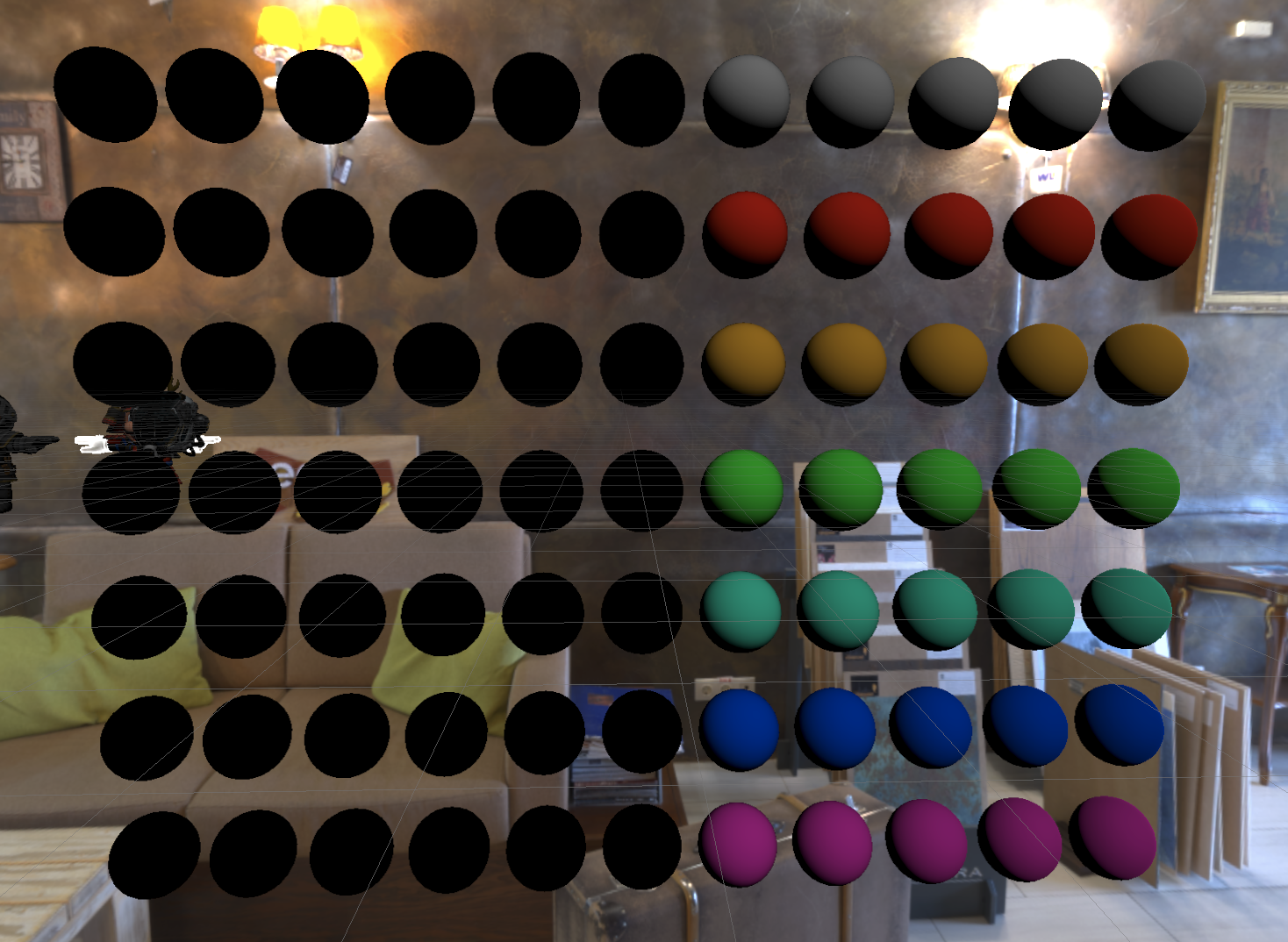
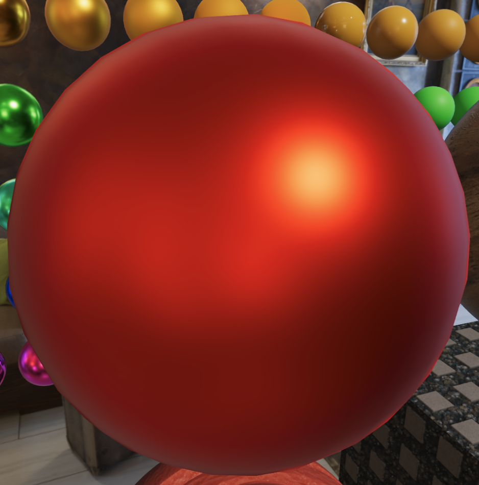
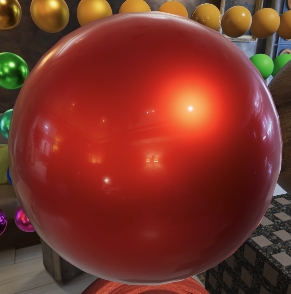
Once we have them done, we can check our direct specular result:

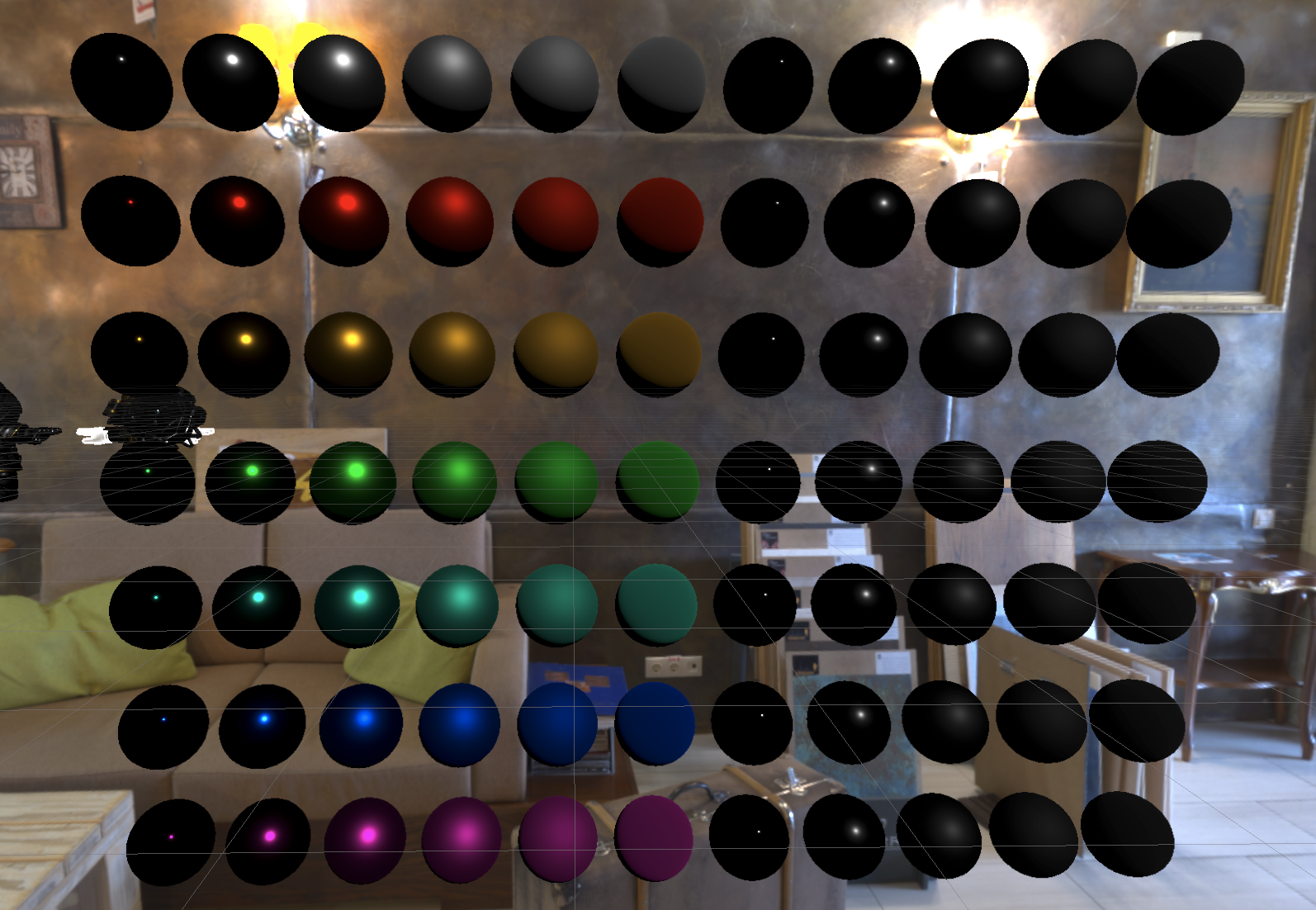
It looks good! … except one problem – the surface becomes darker when having a high roughness value. This is because the specular reflection model we use here is the Cook-Torrance model, which only considers one single bounce of the light. Therefore, when the surface roughness is high or viewing at a grazing angle, the lighting is darker due lacking of multiscattering.

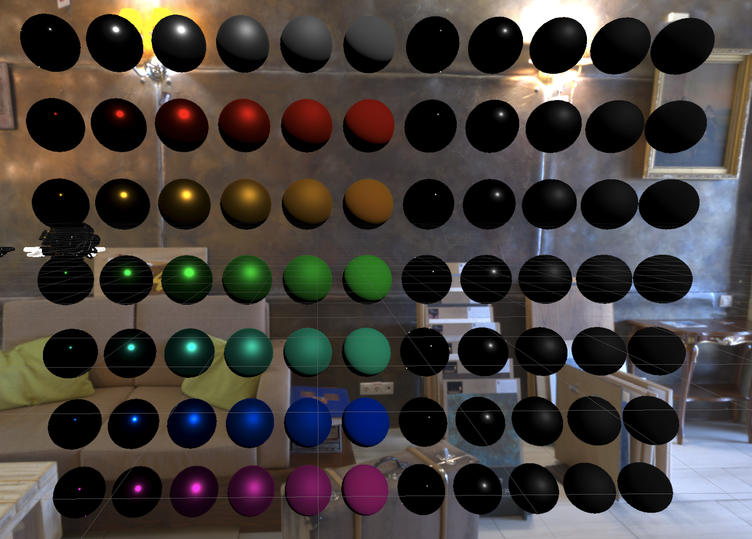
So how do we fix the issue? I implemented the method suggested by Filament. Basically we multiply the specular result with an extra energy compensation term to renormalize the specular lighting. To save computation cost, we store the energy compesation result into the brdf lut generated for the image based lighting (which I’ll go through it later) as this term is dependent on roughness and view angle (NdotV).

float3 CalculateFr(float NdotV, float NdotL, float NdotH, float LdotH, float alphaG2, float3 f0, float3 energyCompensation) {
    float V = V_SmithGGX(NdotV, NdotL, alphaG2);
    float D = D_GGX(NdotH, alphaG2);
    float3 F = F_Schlick(f0, LdotH);
    return D * V * INV_PI * F * energyCompensation;
}

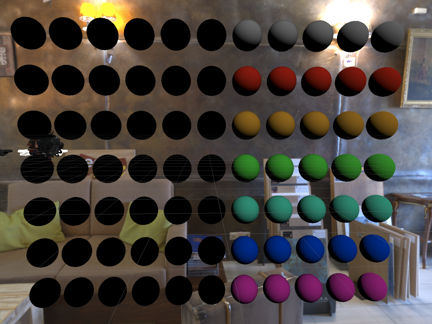
Here’s the result after energy compensation, and you can see rough surfaces are no longer dull:

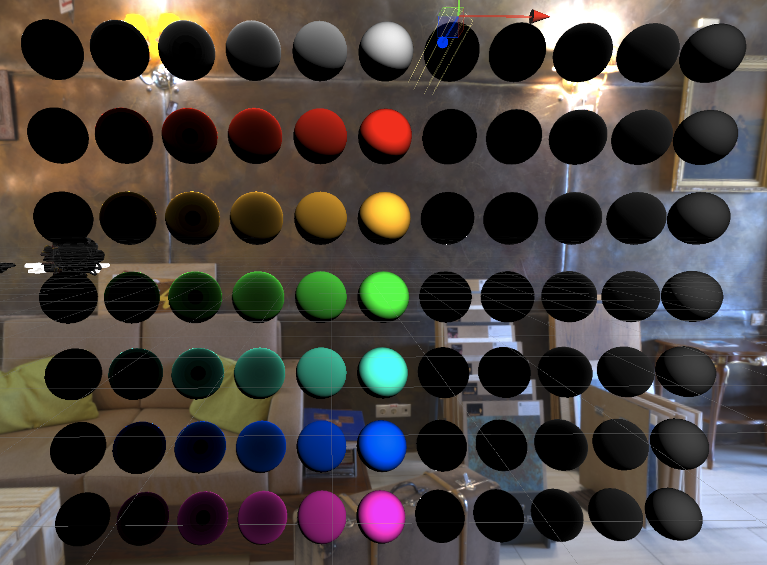
Bonus screenshot on the visualisation of the energy compensation factor (output is energyCompensation - 1.0f since it is a scaling factor):

Indirect Diffuse

Here we will try to capture a one-bounce indirect diffuse lighting. The most common method nowadays is projecting the irradiance information on spherical harmonics, since SH representation takes way less space and is easy to interpolate. However, for the sake of simplicity, I’m using the good old irradiance cubemap, which is basically applying a cosine weighted hemispherical sampling on the environment map. I’m being lazy here. Instead of prefiltering the environment map myself, I directly use the prefilter result provided by Unity. (One main reason I didn’t prefilter myself was because Unity does not support writing to a cubemap in compute shader, which is really weird.) The irradiance map generated by Unity is somewhat blocky and the generation takes a huge amount of time because it happens on CPU (my god). So, probably not a good idea to use that, but anyway.

We use surface normal to sample the irradiance map, multiple with the fresnel term, and then the ambient occlusion factor. The fresnel term here also needs to consider the roughness factor.

float3 F_SchlickRoughness(float3 f0, float u, float linearRoughness) {
    float r = 1.0f - linearRoughness;
    return f0 + (max(float3(r, r, r), f0) - f0) * pow5(saturate(1.0f - u));
}

Indirect Specular

Again, for this part, prefiltering is handled by Unity as for now. A strange thing is that no matter how large the original cubemap is, Unity will only prefilter until the mipmap 6. Therefore, even though I feed in a 2048-res cubemap (which should a max mip level of 11), only mip 0-6 are valid mips. The rest mips (7-11)) are all trash data.

So when we map the roughness to mipmap level, we need to specifiy max mip as 6 instead of 11.

Another issue is how to map roughness to mipmap level. The easiest way of doing this is mip = linearRoughness * maxMip. However, this approximation is far from accurate. Unity offers a better approximation, which is mip = linearRoughness * (1.7f - 0.7f * linearRoughness) * maxMip. This method is accurate enough, though there’s a even more precise way, which you can find it under ImageBasedlighting.hlsl in the core render pipeline package:

// The *accurate* version of the non-linear remapping. It works by
// approximating the cone of the specular lobe, and then computing the MIP map level
// which (approximately) covers the footprint of the lobe with a single texel.
// Improves the perceptual roughness distribution and adds reflection (contact) hardening.
// TODO: optimize!
real PerceptualRoughnessToMipmapLevel(real perceptualRoughness, real NdotR)
{
    real m = PerceptualRoughnessToRoughness(perceptualRoughness);

    // Remap to spec power. See eq. 21 in --> https://dl.dropboxusercontent.com/u/55891920/papers/mm_brdf.pdf
    real n = (2.0 / max(REAL_EPS, m * m)) - 2.0;

    // Remap from n_dot_h formulation to n_dot_r. See section "Pre-convolved Cube Maps vs Path Tracers" --> https://s3.amazonaws.com/docs.knaldtech.com/knald/1.0.0/lys_power_drops.html
    n /= (4.0 * max(NdotR, REAL_EPS));

    // remap back to square root of real roughness (0.25 include both the sqrt root of the conversion and sqrt for going from roughness to perceptualRoughness)
    perceptualRoughness = pow(2.0 / (n + 2.0), 0.25);

    return perceptualRoughness * UNITY_SPECCUBE_LOD_STEPS;
}

Finally, we need to pre-compute a BRDF lut to query DFG at runtime. There are plenty of resources on how to do this. What’s different here is that we also need to take account the specular multiscattering energy compensation. I spent the most time on this part.

To make our BRDF account for multiscattering compensation, I use the method described by Filament:

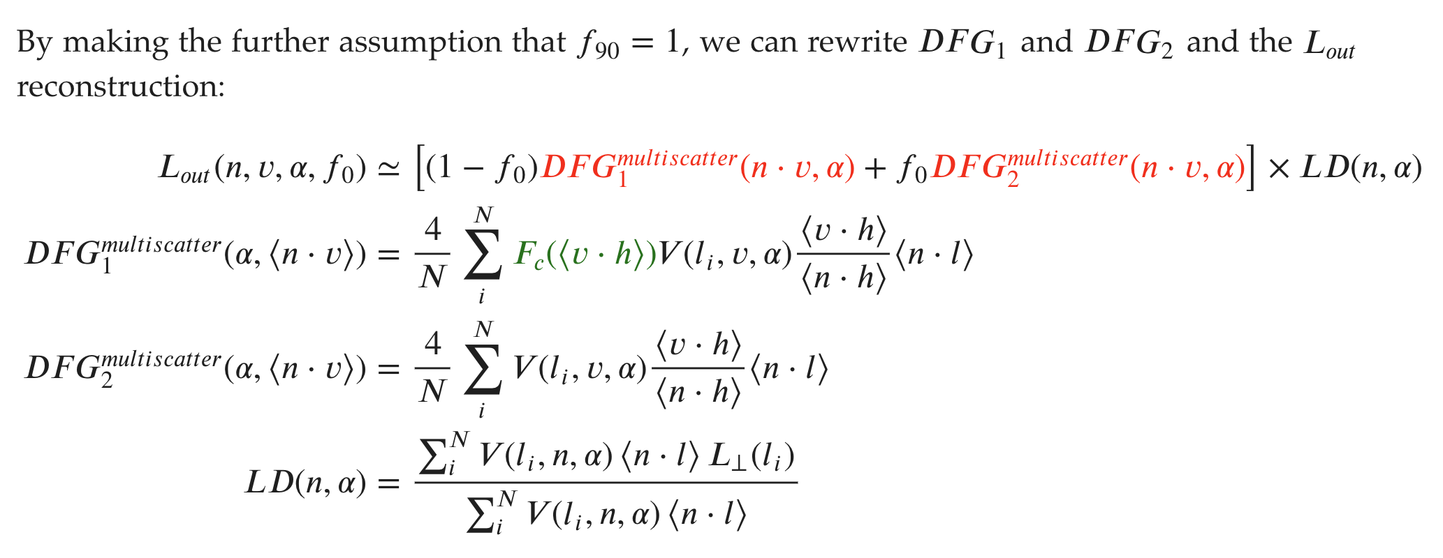
Thus, when we integrate the BRDF lut, we need to add the following lines for each sample:

float G = IBL_G_SmithGGX(NdotV, NdotL, alphaG2);
float Gv = G * VdotH / NdotH;
float Fc = pow5(1.0f - VdotH);
r.x += Gv;
r.y += Gv * Fc;

Here’s the BRDF lut I end up generated (b channel is for diffuse lookup):

u: NdotV [0~1], v: roughness [0~2] (note: roughness, not linear roughness)

I wrote an editor window, which dispatched a compute pass to generate the lut. However, you could also compute this lut at the start of the rendering program as it is fairly quick (less than 1 sec with 1024x1024 resolution). Also, be aware of gamma correction issue. We need to treat this lut as a linear texture.

In addition, when we query the BRDF lut, we should also modfiy the result we get:

float3 CompensateDirectBRDF(float2 envDGF, inout float3 energyCompensation, float3 specularColor) {
    float3 reflectionDGF = lerp(envDGF.ggg, envDGF.rrr, specularColor);
    energyCompensation = 1.0f + specularColor * (1.0f / envDGF.r - 1.0f);
    
    return reflectionDGF;
}

And we need to multiply the indirect specular result with the energyCompensatin term.

Specular Miscs

Right now wew can already see the power of full PBR. However, there are a few points I haven’t mentioned yet.

First, we need to clamp the minimum value of linear roughness. One reason is to reduce specular aliasing (which is not the only method). Another reason is to prevent float point inaccuracy when compute roughness (even smaller than linear roughness). I clamp the value to 0.045. If you’re on mobile platform, you probably want to rise the bar to 0.089 due to half precision (according to Filament).

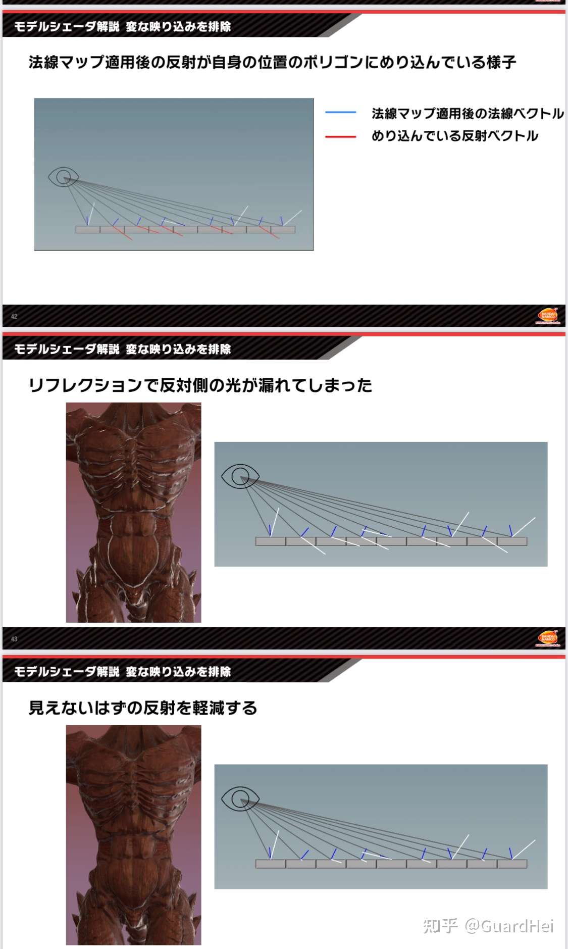
The other thing is that we have to deal with occlusion of indirect lighting. I don’t have any specular ao or bent normal map, as well as implementing any screen space occlusion technique, so we gonna use some easy tricks here. For indirect diffuse, we simply multiply with AO map which is mostly enough. For indirect specular, I use the Horizon Specular Occlusion method seen in Super Smash Bros: Ultimate, which is firstly introduced by Marmoset.

One problem that causes indirect specular light leaks is because the normal map may rotate the surface normal back towards the model itself. In this case, the model itself should occlude the indirect specular lighting.

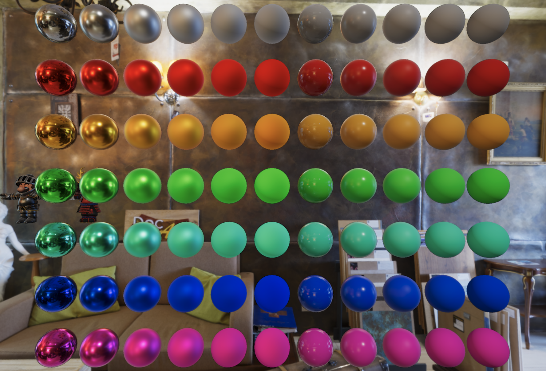
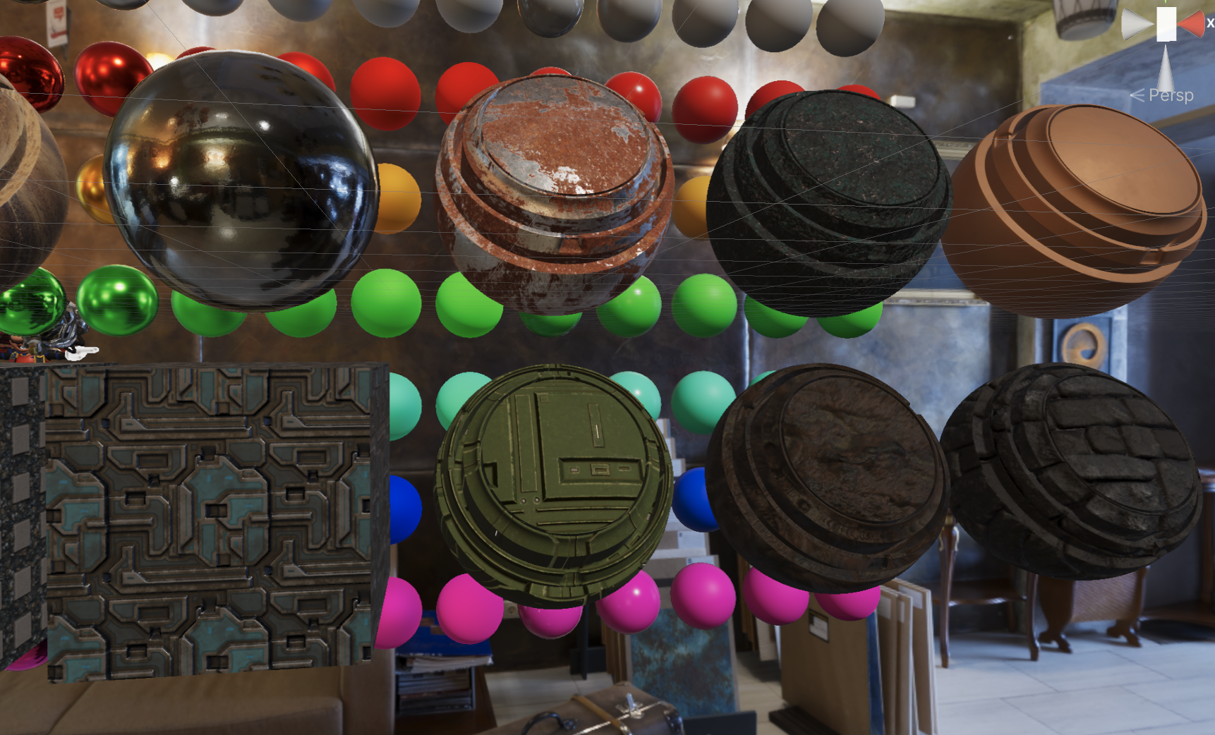
And that’s the basic PBR. Finally, we add up direct lighting, indirect lighting, as well as emission values, and apply a ACES Tonemapping to map HDR lighting result to SDR display range. This is what we got:

Damaged Helmet (glTF 2.0)

PBR Spheres

Here’s the visualization of the Horizon Specular Occlusion:

Final Lighting Result

Horizon Specular Occlusion Factor

Indirect Specular Result

More PBR

After implementing the standard PBR materials, we can extend the framework to include more special materials, including clear coating, anisotropic specular, fabric, and etc.

Before, we need to modfiy our shader structure. I extract the skeleton of the code but encode them using MACROs so that I don’t have to copy & paste a bunch of property set up code every time I want to write a new material. Kinda like the idea of Surface Shader brought by Unity a while ago, but we don’t have any editor support. The downside is that writing shaders in MACRO lacking support from IDE editor – there’s no auto complete, no syntax check. But anyway it works.

Clear Coating Material

I basically follow Filament’s idea here. To put it simple, we add another specular lobe layer for the clear coating on top of the original specular lobe. We also need to multiply the base layer with a loss term to make sure energy conservation. The extra specular lobe has the same computation as the base layer. Yet Filament changed the visibility term to V_Kelemen. Why? Because it’s cheap, and roughness doesn’t affect too much for clear coating layer, we can safely discard it.

float V_Kelemen(float LdotH) {
    return .25f / max(pow2(LdotH), .00001f);
}

There ain’t much else to say, besides a bunch of details. First, because clear coating is an extra layer on top of the original surface, there shouldn’t be too many geometric details. Thus, to suppress the subtle details, we choose to use the original vertex normal instead of the one we get after modified by the normal map. Then, this extra layer will also change the f0 of the base layer, so we need to apply the following modification:

// This is a fitting assuming clear coating layer has a IOR of 1.5
float3 F0ClearCoatToSurface(float3 f0) {
    return saturate(f0 * (f0 * (.941892f - .263008f * f0) + .346479f) - .0285998f);
}

In addition, the clear coating layer will also affect the roughness of the base layer. Technically we should compute this using IOR. However, we are again playing simple here, clamping the roughness of the base layer to the roughness of the clear coating layer.

linearRoughness = lerp(linearRoughness, max(linearRoughness, linearClearCoatRoughness), clearCoat);

Two layers of specular lobes also means two times the indirect specular sampling. The render pipeline I’m working on is a forward+ one, so I don’t have to care about how to compress all these extra parameters (clear coat strength and clear coat roughness) into the GBuffer if we are using deferred rendering. We simply sample the indirect specular of the clear coating layer in the forward lighting pass, and output the base layer’s f0 to a thin-GBuffer (so that we can mix the result with screen space reflection). The downside is that clear coat layer won’t have SSR, but it isn’t a big deal, plus you can swap the base layer and the clear coat layer to see which one has a smaller visual impact

And here are the results:

Clear Coat = 0 (Metallic = 1, Smoothness = .5)	Clear Coat = 1 (Metallic = 1, Smoothness = .5)

I really like clear coating material, probably because a photo I took last year:

I call this Chinese Cyberpunk

Anisotropic Specular Material

I use the method described in Far Cry 4. The core code snippets are here:

// the stretching of the specular, normally 5.0f, but we can have artists adjust it.
const float stretch = 5.0f;

float3 anisotropyDirection = (anisotropy >= .0f) ? B : T.xyz;
float3 anisotropicT = cross(anisotropyDirection, V); 
float3 anisotropicN = cross(anisotropicT, anisotropyDirection);
float anisotropyFactor = abs(anisotropy) * saturate(stretch * linearRoughness);
float3 bentNormal = normalize(lerp(N, anisotropicN, anisotropyFactor));

And we get the results:

Anisotropy = 0	Anisotropy = 1

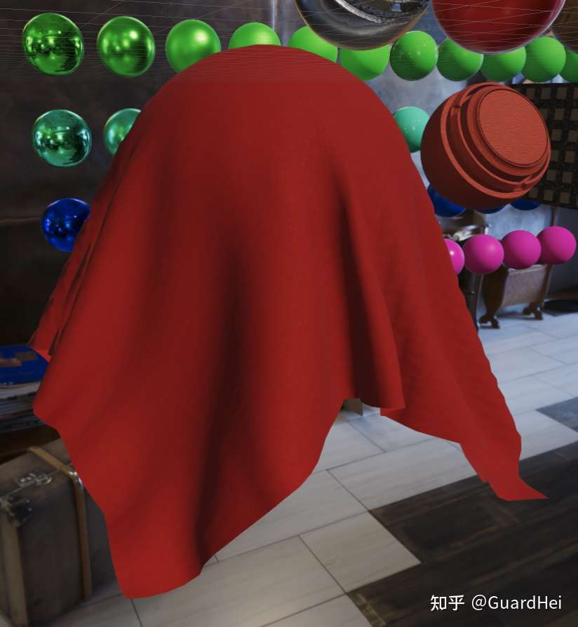
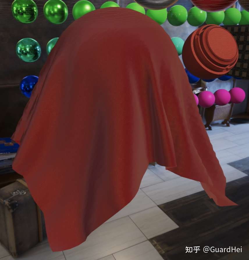
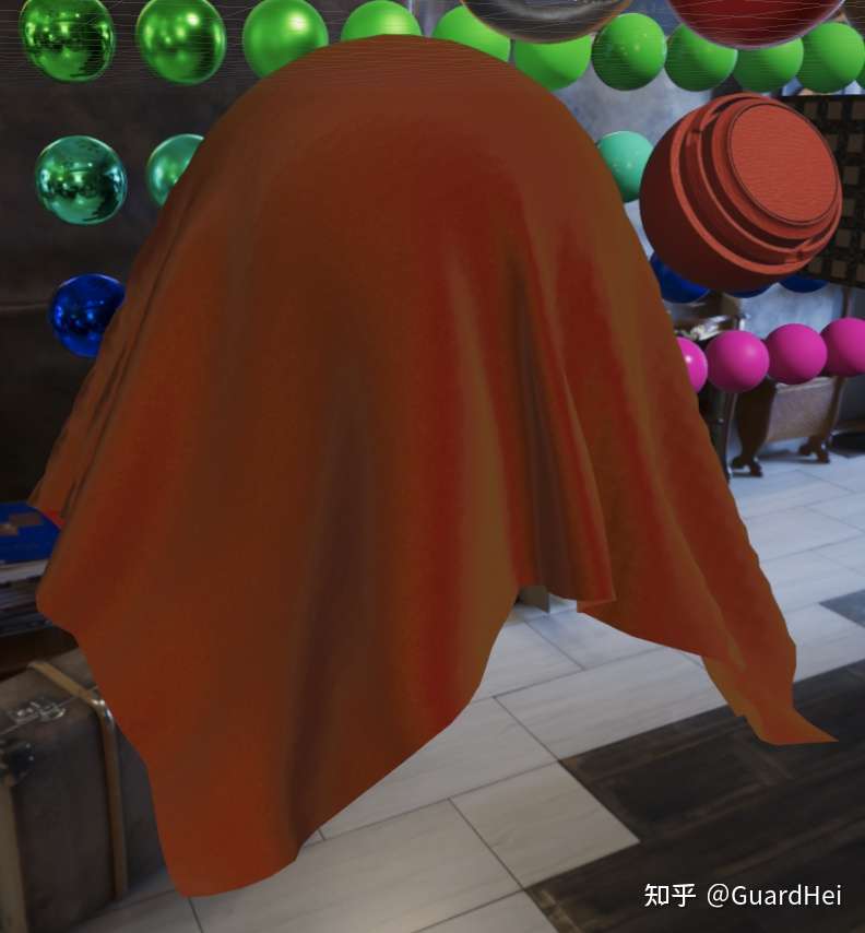
Fabric Material

Filament has a good summary of Fabric, but I did it differently.

First there is the direct diffuse. We replace our multiscatter diffuse with a empirical model based on Lambertian model, so that it won’t be too bright.

// From Unity renderpipeline.core（but it's probably from somewhere else）
// Caller needs to div by PI
float3 FabricLambertDiffuse(float roughness, float3 diffuse) {
    return lerp(1.0f, .5f, roughness) * diffuse;
}

Yet the back face is too dark. Thus, we need to simulate the subsurface scattering effect. Here we use a simplified hack to achieve a similar visual result. Instead of using saturate(NdotL), we use:

float3 directDiffuse = fd * saturate((NdotL + .5f) / 2.25f); // The later part is actually saturate((NdotL + w) / (1.0 + w) * (1.0 + w))，we assume w=0.5f，but it could be exposed to the artists
directDiffuse *= saturate(mat.subsurfaceColor + float3(NdotL, NdotL, NdotL)) * light.color;

Then there’s the direct specular, which we need to change the D term and the V term to achieve the forward and backward sacttering effect of the fabric.

The common choices of D() and V() are from Ashikhmin07. However, after Imageworks published this article, people generally changed D() to D_Charlie.

// Mainly from Filament, prevent div by 0 on half precision floating point

// Caller needs to div by PI
// Ashikhmin 2007, "Distribution-based BRDFs"
float D_Ashikhmin(float NdotH, float alphaG2) {
    float cos2h = NdotH * NdotH;
    float sin2h = max(1.0f - cos2h, .0078125f); // 2^(-14/2), so sin2h^2 > 0 in fp16
    float sin4h = sin2h * sin2h;
    float cot2 = -cos2h / (alphaG2 * sin2h);
    return 1.0f / ((4.0f * alphaG2 + 1.0f) * sin4h) * (4.0f * exp(cot2) + sin4h);
}

// The popular method now, faster and better
// Caller needs to div by PI
// Estevez and Kulla 2017, "Production Friendly Microfacet Sheen BRDF"
float D_Charlie(float NdotH, float roughness) {
    float invAlpha  = 1.0f / roughness;
    float cos2h = NdotH * NdotH;
    float sin2h = max(1.0f - cos2h, .0078125f); // 2^(-14/2), so sin2h^2 > 0 in fp16
    return (2.0f + invAlpha) * pow(sin2h, invAlpha * .5f) * .5f;
}

However, most people still use V_Ashikhmin() for visibility term, including Unreal 4.

// The result is good enough tbh
float V_Ashikhmin(float NdotL, float NdotV) {
    return saturate(1.0f / (4.0f * (NdotL + NdotV - NdotL * NdotV)));
}

Unity HDRP has implemented V_Charlie, but it’s only used in pre-integrating the BRDF lut for the specular IBL, not the runtime computation for direct specular due to higher cost. Also, the original paper has a Terminator Softening term to allow smoother transition for the visibility term (not physically correct, but artists love it), which is not implemented by Unity.

Therefore, here’s the V_Charlie we gonna use at last:

float CharlieL(float x, float r) {
    r = saturate(r);
    r = 1.0f - pow2(1.0f - r);

    float a = lerp(25.3245f, 21.5473f, r);
    float b = lerp(3.32435f, 3.82987f, r);
    float c = lerp(.16801f, 0.19823f, r);
    float d = lerp(-1.27393f, -1.97760f, r);
    float e = lerp(-4.85967f, -4.32054f, r);

    return a / (1.0f + b * PositivePow(x, c)) + d * x + e;
}

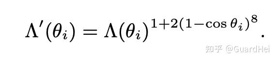
float SoftenCharlie(float base, float cos_theta) {
    const float softenTerm = 1.0f + 2.0f * pow8(1.0f - cos_theta);
    return pow(base, softenTerm);
}

float V_Charlie_No_Softening(float NdotL, float NdotV, float roughness) {
    const float lambdaV = NdotV < .5f ? exp(CharlieL(NdotV, roughness)) : exp(2.0f * CharlieL(.5f, roughness) - CharlieL(1.0f - NdotV, roughness));
    const float lambdaL = NdotL < .5f ? exp(CharlieL(NdotL, roughness)) : exp(2.0f * CharlieL(.5f, roughness) - CharlieL(1.0f - NdotL, roughness));
    return 1.0f / ((1.0f + lambdaV + lambdaL) * (4.0f * NdotV * NdotL));
}

float V_Charlie(float NdotL, float NdotV, float roughness) {
    float lambdaV = NdotV < .5f ? exp(CharlieL(NdotV, roughness)) : exp(2.0f * CharlieL(.5f, roughness) - CharlieL(1.0f - NdotV, roughness));
    lambdaV = SoftenCharlie(lambdaV, NdotV);
    float lambdaL = NdotL < .5f ? exp(CharlieL(NdotL, roughness)) : exp(2.0f * CharlieL(.5f, roughness) - CharlieL(1.0f - NdotL, roughness));
    lambdaL = SoftenCharlie(lambdaL, NdotL);
    return 1.0f / ((1.0f + lambdaV + lambdaL) * (4.0f * NdotV * NdotL));
}

CharlieL() function is essentially doing a lut interpolation. Imageworks has already done the fitting for the 5 coefficients (abcde) when r = 0 and r = 1. Then we use (1 - r) ^ 2 to interpolate.

Terminator softering is a power operation, I’ve implemented a fast pow8() function.

V_Charlie does not bring a huge improvement. It mainly suppresses the over-brightness part at grazing angle compared to V_Ashikhmin. Terminator softening is also very subtle. At the same time, the cost of V_Charlie plus terminator softening is way too high and probably don’t worth the performance cost.

Then there’s the Fresnel term. We don’t need to change the function itself, but we want to pass in a separate sheen parameter instead of the original f0 – basically manually assigning the specular color. I’m kinda confused by what Filament does here. It seems Filament direct assign sheenColor without doing the Fresnel computation. Not sure why, so I followed Unreal’s method here.

In addition, we need to modify the indirect specular, especially the BRDF lut computation since V and D have changed. I don’t get much time so kinda ignore it for now.

This is what I get in the end:

Original PBR	Velvet Fabric PBR	Velvet Fabric PBR with Green Sheen

PS: Not sure why when exporting the cloth mesh as .fbx from Maya, it gonna lose all the cloth simulation info. And it does not happen if I exported it in .obj. Weird.

AND MORE AND MORE

There’re still plenty more PBR models to implement, such as more accurate subsurface scattering, or iris specular. It is really satisfying to collect different BxDF models from place to place. Well, I guess that’s it for now.